Calculating Stormwater Peak Discharge From Small Catchments
This article presents a procedure for calculating stormwater peak discharge from small catchments in Albuquerque, NM, that is based largely on standard Natural Resources Conservation Service (NRCS) rainfall-runoff methods whereby rainfall excess from a 24-hour design storm is determined using the curve-number approach and is then transformed to runoff by means of a triangular unit hydrograph. The single departure from standard NRCS calculations is use of a design storm developed specifically for Albuquerque using up-to-date precipitation frequency data. The NRCS procedures are then encapsulated concisely in the form of graphs based on normalized solution parameters, and mathematical expressions that approximate the graphs closely, to obtain numerically reliable estimates of peak flow rates from small catchments in a very straightforward way. Maximum rainfall intensities contained within the local Albuquerque design storm are considerably greater than those in the standard NRCS storm that applies to the region, which results in calculation of significantly larger peak discharges from small catchments. The procedure provides an alternative to the rational formula that takes into account land use/land cover conditions, soil infiltration characteristics, and rainfall intensity, which serves as a proxy for the influence of return period on the peak runoff relation.
A dimensionless unit hydrograph of triangular shape developed by the NRCS, which is based on a large number of unit hydrographs from basins of various sizes and geographic locations, is used often to generate storm runoff hydrographs from small catchments (NRCS 2007b, page 16-2 and Appendix 16A). Usually applied in combination with standard 24-hour storm patterns and the runoff curve-number (CN) approach to estimate rainfall losses, the triangular unit hydrograph provides a straightforward means of calculating runoff hydrographs needed to design structural and non-structural measures used to control both the quantity and quality of stormwater runoff.
Design of some minor hydraulic structures (for example, side or median ditches for roadway drainage, closed storm sewers and their inlets that convey stormwater runoff, roadway culverts and small bridges, and stream bank protection works) requires only the peak discharge from a catchment and typically not a complete storm runoff hydrograph. In such circumstances, the NRCS rainfall-runoff calculation procedure can be used to determine the required peak discharge without computing an entire runoff hydrograph.
Applying the CN approach to determine rainfall excess from 24-hour duration storms based on a temporal distribution developed specifically for Albuquerque, NM, storm runoff is generated by means of the triangular unit hydrograph. Calculations are carried out using normalized solution variables, from which graphical display of a dimensionless measure of peak discharge are acquired. Equations fitted to the graphical relations provide suitable matches to the rigorous numerical solutions, which eliminates the need to carry out time-consuming rainfall-runoff calculations when only peak discharge, and not complete storm runoff hydrographs, are needed.
NRCS Rainfall-Runoff Relations
NRCS rainfall-runoff relations, which have become de facto national standards for stormwater analysis in the United States, are often used to calculate rainfall-runoff from small watersheds. The procedure is summarized as follows: Rainfall excess obtained using the CN approach applied to 24-hour design storms is transformed to runoff by means of a triangular unit hydrograph. These practices are described briefly to provide background for the analysis that follows. More thorough explanations are given in NRCS (1986, 2004a, 2004b, 2007a, 2007b, 2009), McCuen (1998), and Hawkins et al. (2009).
Rainfall Distributions. Rainfall patterns for storms of 24-hour duration have been prepared by the NRCS for four geographic regions of the United States using rainfall depths for storm durations from 6 minutes to 24 hours in increments of 6 minutes obtained from the US Weather Bureau’s “Rainfall Frequency Atlas of the United States” (Hershfield 1961), which is widely known as Technical Paper 40 (TP-40). For each storm type, a series of incremental rainfall depths ranked from largest to smallest was found by subtracting 6-minute depths from 12-minute depths, then subtracting 12-minute depths from 18-minute depths, and so on up to the 24-hour depths. The incremental rainfall depths were then distributed within the 24-hour period centered about the time of peak intensity, which is based on recorded storms, so that the maximum 6-minute depths are contained within the maximum 12-minute depths, which are contained within the maximum 18-minute depths, and so on (McCuen 1998, pages 204-205). As a consequence of the storm construction procedure, average rainfall intensities for all durations less than 24 hours are contained within the NRCS distributions.
The NRCS synthetic design storms are presented as ratios of cumulative rainfall depth to total rainfall depth as functions of time. The author (Froehlich 2009, 2010) provides a mathematical expression that approximates the tabulated NRCS rainfall distributions closely as follows:
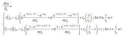
where P(t) = cumulative rainfall depth, t = time since the start of rainfall in hours, td = storm duration in hours (which is 24 hours for the standard NRCS storms), P24 = 24-hour rainfall depth, r = time-to-peak rainfall intensity ratio (0 ≤ r ≤ 1), η′ = 1- η, and ip*, io*, η, m1, and m2are coefficients found for each of the four NRCS storm types. The storm pattern places 100 × r percent of total storm rainfall before the peak intensity at time t = r × td, and 100 × (1 – r) percent after the peak. With r = 0 (that is, considering the peak intensity to occur at the start of rainfall), Equation (1) reduces to:
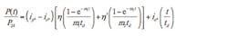
which provides a relation giving the maximum t-minute duration precipitation at time t. Viewed in another way, Equation (2) provides a mathematical representation of commonly used precipitation depth-duration relations with the largest intensity at t = 0.
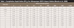
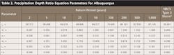
The same approach used to develop the standard NRCS storms based on rainfall data obtained from TP-40 is applied here to create 24-hour design storms specifically for Albuquerque based on recent precipitation depth ratios (that is, P/P24) for various durations and return periods obtained from the National Oceanic and Atmospheric Administration (NOAA) Atlas 14 (Bonnin et al. 2006), which are presented in Table 1. Design storm coefficients found by fitting Equation (2) to the precipitation depth ratios for each return period are given in Table 2.
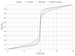
Design storm distributions given by Equation (1) with r = 0.5 (that is, peak intensity of each storm is considered to occur at t = 12 h for each storm pattern) for 2-, 10-, and 100-year return periods are shown in Figure 1 along with the standard NRCS Type 2 storm (which is the NRCS storm type that applies to the entire state of New Mexico.) From the figure, cumulative rainfall distributions created specifically for Albuquerque are shown to differ significantly from the NRCS Type 2 storm, producing peak intensities (which are given by the largest slope of a curve) that are from 70% to 80% greater than the Type 2 storm peak. Also evident from Figure 1, the 10-year, 24-hour rainfall distribution provides a good average for all return period design storms. For this reason, the following analysis uses a dimensionless storm pattern that is based on the 10-year, 24-hour Albuquerque design storm.
Rainfall Excess. The NRCS procedure for estimating rainfall excess accounts for total storm rainfall P by dividing it into three components: direct runoff Q, actual rainfall retention during a storm F, and the initial abstraction Ia (NRCS 2004b, pages 10-2 to 10-4; Hawkins et al. 2009, pages 6–9). The physical unit of each of these quantities is rainfall volume per unit area (rainfall depth). The conceptual relation between P, Q, F, and Ia is given by:
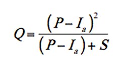
where S = the potential maximum retention. It is generally accepted and in part shown in some empirical studies that initial abstractions are related to retention as Ia = kaS, where ka ≈ 0.2, although wide variation of ka has been found (Hawkins et al. 2009), is a dimensionless coefficient. Potential maximum retention is calculated as
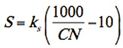
where ks = retention depth units conversion factor (1.0 for S in inches, 25.4 for S in mm), and CN = runoff curve number = an index ranging theoretically from 0 to 100 (a larger CN indicates greater runoff potential), although in practice usually 40 ≤ CN ≤ 98.
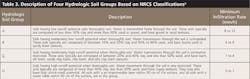
CN represents the combined effect of soil type, land use, and land cover (vegetation types, degree of imperviousness, and agricultural treatments). Soils are classified by hydrologic soil group (HSG), that is, a group of soils having similar runoff potential under similar storm and cover conditions (NRCS 2007a). The NRCS has placed more than 4,000 soils into four hydrologic groups (A, B, C, and D) whose runoff potential ranges from low to high as described in Table 3. HSG classification is made based on similarities of soil hydrologic and physical properties, under the premise that saturated soils with similar depth, permeability, and texture will have similar response during an intense rainstorm.
Watershed surface conditions are characterized by land use and treatment classes. Land cover includes every kind of vegetation, litter and mulch, fallow, and bare soil as well as nonagricultural uses, such as water surface (lakes, swamps) and impervious surfaces (roads, roofs). Land treatment, which applies primarily to agricultural watersheds, includes mechanical practices, such as contouring or terracing, and management practices, such as grazing control or rotation of crops. A combination of HSG (soil) and a land use and treatment class (cover) is known as a hydrologic soil-cover complex. Tables and graphs of CN assigned to such complexes have been prepared for agricultural and urban watersheds (NRCS 2004a).
Triangular Unit Hydrograph. A dimensionless curvilinear unit hydrograph developed by the NRCS, which has 3/8 of the total runoff volume in the rising side, is resembled closely by a triangle (NRCS 2007b, Appendix 16A; McCuen 1998, pages 535-536). For the triangular approximation (Figure 2), kr = tr/tp = 5/3 (the average value found by the NRCS), where tp = time-to-peak = time between the beginning of runoff from a short high-intensity storm and the corresponding peak rate of runoff from the catchment, and tr = recession time = time from hydrograph peak flow to the end of direct runoff. The ratio kr might vary depending on watershed topography, the amount of impervious land cover, and the extent to which natural stream channels have been replaced by storm sewers.
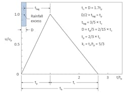
Based on the triangular approximation, the unit hydrograph peak discharge up (that is, the peak discharge resulting from an amount of excess rainfall Q = 1 unit applied uniformly over the catchment within a specified rainfall duration D) from a catchment of area A is found as
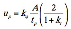
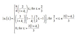
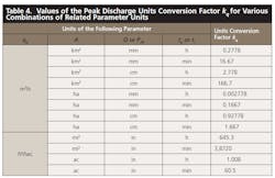
where kq = units conversion factor that depends on the units of up, A, Q, and tp (Table 4.) Evaluation by the NRCS of hydrographs from a large number of watersheds provided typical values of D = tp/5 and tp = 2/3 × tc, where tc = time-of-concentration of a catchment. The mathematical representation of the triangular unit hydrograph is then
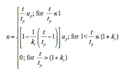
where t = time since the start of runoff.
Runoff Hydrograph Calculation. The linear response of a catchment to unit pulses of excess rainfall is given by the discrete convolution integral (Chow et al. 1988, pages 211–213) as
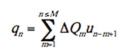
where qn = outflow at t = nD, ΔQm = Qm – Qm-1 = incremental direct runoff during the mth time interval, and Qm = Q given by Equation (3) for P(t = mD) obtained from Equation (1). Input to Equation (7) is a series of M values of ΔQ. When using 24-hour duration design storms, M = 24/D, where D is in hours, although ΔQ = 0 for P ≤ Ia.
Dimensionless Runoff Formulation
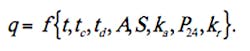
Making use of Equation (1) to obtain incremental rainfall depths, Equation (3) to obtain rainfall excess (that is, the incremental runoff depth), and Equation (6) to describe the unit hydrograph for a unit rainfall duration D = 2/15 × tc, outflow from a catchment is given by the following functional relation for a particular rainfall distribution:
By creating a set of dimensionless parameters, the number of variables in Equation (8) can be reduced, and the task of calculating runoff made less complicated. Using appropriate combinations of tc, td, P24, and A to normalize the remaining variables, the following dimensionless functional relation results:
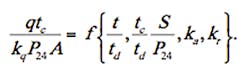
For specified values of ka and kr, Equation (9) reduces to
where
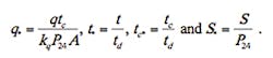
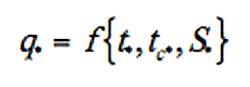
Because storm duration td = 24 h is constant for the following analysis, and because time distributions of q* are not needed if only peak discharge is of interest, the functional relation for qp*, the maximum value of q*, is then
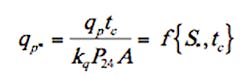
that is, qp* depends on only two variables, S* and tc. As a result, the relation for qp* can be graphed in a clear and uncomplicated way, thereby providing a straightforward and rapid means of finding the peak rate of runoff from a small catchment.
The dimensionless discrete convolution integral for q* is
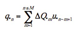
where ΔQ*m = Q*m – Q*m-1, and Q*m = Qm/P24. From Equation (3),
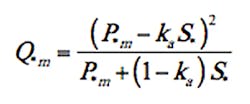
where P*m = P(t=mD)/P24. Combining Equations (5) and (6), and recalling that tp = 2/3 × tc, gives
Remembering that D=2/15 × tc, the dimensionless time t* =t/tc = nD/tc = 2n/15, which gives u*n = u*(t*=2n/15).
Graphical and Mathematical Relations for qp*
Accurate numerical solutions for qp* were obtained from Equation (14), with the assistance of Equations (15), (16), and (2), using the dimensionless Albuquerque design storm (which is based on the 10-year return period storm pattern) for all combinations of S* (ranging from 0 to 3 by increments of 0.01) and tc (5, 10, 15, 20, 30, 45, 60, 90, and 120 min) with kr = 5/3 and ka = 0.2 (that is, using the NRCS standard values of ka and kr.) Computed values of qp* are graphed against S* for the several values of tc evaluated in Figure 3.
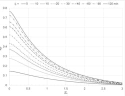
Curves of qp* for a particular value of tc in Figure 3 were created by connecting the calculated values by a series of straight lines. For this reason, there is no scatter of solution points about the curves, which are exact solutions for all practical purposes. Exactness of a graphical estimate of qp* depends only on the precision of the interpolated value.
The straightforward expression that follows provides accurate estimates of calculated values of qp* used to construct the graphs in Figure 3:
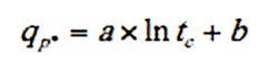
where
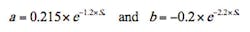
and tc is in minutes. The coefficient of determination of Equation (16) is 0.998, and the standard error of estimate is 0.00715. Differences between the graphical solutions for qp* and approximations given by Equation (16) are largest when S* ≈ 0 (that is, when the catchment is nearly completely impervious), and for tc < 10 min, never exceeding 5%. Because the 10-year, 24-hour rainfall distribution provides a good average for all return period design storms, the graphical and mathematical relations for qp* can be used to estimate reliably the peak discharge for any other return period typical in hydrologic design of minor hydraulic structures.
Example Application
An example is presented to illustrate use of the procedures presented here to calculate qp at the outlet of a small catchment located near Albuqurque for a range of return periods (2 to 1,000 years). The watershed is undeveloped, with less than 30% of the nearly flat drainage area covered by sagebrush with grass understory. Watershed parameters are as follows: A = 113 ha, tc = 1.5 h = 90 min, and CN = 67 for HSG B soils that typify the Albuquerque area, which gives S = 125 mm from Equation (4).
Combining Equations (16) and (12) gives qp as follows:
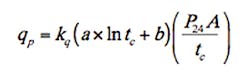
With values of P24 obtained from NOAA Atlas 14 (Bonnin et al. 2006), S* = S/P24 is calculated first, the coefficients a and b are then found from Equation (17), and finally qp is given by Equation (18), with kq = 0.1667 from Table 4 for qp in m3/s, P24 in mm, A in ha, and tc in min. All calculations based on NRCS rainfall-runoff calculation using a design storm created specifically for Albuquerque from NOAA Atlas 14 precipitation data that are encapsulated in Equation (18) are summarized in Table 5. Also included in Table 5 are the peak discharges obtained from conventional application of the NRCS rainfall-runoff calculation procedure using the standard Type 2 design storm, which is developed from precipitation data from TP-40. Peak discharges computed by both approaches are graphed as a function of return period in Figure 4.
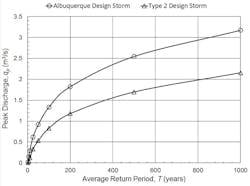

As shown in Figure 4, peak discharges determined using the rainfall distribution developed specifically for Albuquerque from NOAA Atlas 14 precipitation data are significantly greater than those obtained from standard NRCS calculations based on the Type 2 design storm. The percentage increases are particularly large for small return periods. For T = 100 years, the peak discharge given by Equation (18) is 60% greater than the value obtained from conventional calculations using the Type 2 design storm. This comparison emphasizes the need to develop local design storms from up-to-date information because peak rainfall intensities can vary significantly from those given by the standard NRCS rainfall patterns.
Summary and Conclusions
A procedure is presented for calculating stormwater peak discharge from small catchments in Albuquerque that is based on standard NRCS rainfall-runoff computation methods, making use of a 24-hour design storm developed specifically for Albuquerque. Accurate numerical solutions for dimensionless peak discharge qp* were obtained by generating dimensionless runoff hydrographs for various combinations of S* (ranging from 0 to 3 by increments of 0.01) and tc (5, 10, 15, 20, 30, 45, 60, 90, and 120 minutes) with kr = 5/3, ka = 0.2 (that is, using the standard values of ka and kr.) Computed values of qp* were graphed against S* for the several values of tc by connecting the calculated values with a series of straight lines. For this reason, there is no scatter of solution points about the curves, which represent the exact solution for all practical purposes. As a result, the entire solution for qp* procedure is reduced to easy to use graphical relations. Mathematical expressions fit to the graphical relations for qp* provide good approximations with differences never exceeding 5%.
The graphical relations and mathematical expressions developed from the rainfall-runoff calculations predict peak discharge based on climatic factors (that is, rainfall intensity through S* = S/P24, which decreases as P24 increases, and design storm patterns, both of which add a geographic influence), the hydrologic soil-cover complex (characterized by CN or S, which account for the effects of land use, vegetative cover, and soil type), and, to a lesser degree, on tc, which is inversely related to rainfall intensity. However, the solution is limited to comparatively small watersheds where runoff can be estimated by standard NRCS hydrologic procedures without having to subdivide the catchment.
Because the computational procedure depends on use of dimensionless design storm patterns that apply regionally, the article focuses on use of the method in Albuquerque. Design storms were developed for the Albuquerque area based on rainfall intensity-duration data obtained from the recently published NOAA Atlas 14 using the same approach applied by the NRCS to develop their standard design storm patterns from rainfall data contained in TP-40. A particularly important finding of the analysis is the large difference between the design storm pattern developed for Albuquerque using up-to-date rainfall data and the NRCS Type 2 storm pattern that applies to the region. As shown in the example application, the larger rainfall intensities contained in the Albuquerque design storm will produce substantially larger peak discharges from small catchments. Consequently, the hydraulic capacity of minor hydraulic structures sized using standard NRCS computation procedures will be exceeded far more often than desired.
Although the approach is used here to calculate runoff from small catchments in Albuquerque, the same procedure can be developed for any location where NRCS rainfall-runoff methods apply, and where precipitation intensity-duration information is available. A case in point is the finding by Vaššová (2013) that the method described by Froehlich (2012) predicts more accurately peak discharges from a small experimental catchment in the Czech Republic than all other techniques evaluated in the comparison study. Finally, the method provides an alternative to the commonly used rational formula for calculating peak discharge that can cope better with variable conditions such as soil type, land cover, and climatic conditions through use of the curve number procedure to obtain rainfall excess, and the unit hydrograph approach to model catchment runoff.
List of Symbols and Abbreviations
A = catchment area
a and b = coefficients in Equation (16) for qp*
CN = runoff curve number
D = unit hydrograph rainfall duration
F = actual rainfall retention during a storm, in volume per unit area or depth
Ia = initial abstract depth, in volume per unit area or depth
io* = rainfall intensity equation coefficient (dimensionless)
ip* = rainfall intensity equation coefficient (dimensionless)
ka = Ia/S = initial abstraction depth ratio
kq = units conversion factor
kr = tr|tp = ratio of triangular unit hydrograph recession time to time-to-peak
ks = retention depth unit conversion factor
m1, m2 = rainfall intensity equation coefficients, in dimensionless m2 units per hour
P = total rainfall or potential maximum runoff; in volume per unit area or depth
P24 = 24-hour storm rainfall depth
Q = direct storm runoff, in volume per unit area or depth
q = flow rate, in volume per unit time
qp = peak discharge from a catchment
qp* = (qptc)/(kqP24A) = dimensionless peak discharge from a catchment
r = time-to-peak rainfall intensity ratio
S = potential maximum retention depth
S* = S/P24 = normalized potential maximum retention depth
T = return period, or average recurrence interval, in years
t = design storm time since start of rainfall
tc = catchment time-of-concentration
td = design storm duration
tr = unit hydrograph recession time
u = unit hydrograph discharge
up = unit hydrograph peak discharge
η = rainfall intensity equation coefficient (dimensionless)
η′ = 1 – η = rainfall intensity equation coefficient (dimensionless)
References
Bonnin, G. M., D. Martin, B. Lin, T. Parzybok, M. Yekta, and D. Riley. 2006. “Precipitation-Frequency Atlas of the United States, Volume 1, Version 4.0: Semiarid Southwest (Arizona, Southeast California, Nevada, New Mexico, Utah).” NOAA Atlas 14– Vol. 1, US Department of Commerce, National Oceanic and Atmospheric Administration, National Weather Service, Silver Spring, MD.
Chow, V. T., D. R. Maidment, and L. W. Mays. 1988. Applied Hydrology. McGraw-Hill, New York, NY.
Froehlich, D. C. 2009. “Mathematical Formulations of NRCS 24-Hour Design Storms.” Journal of Irrigation and Drainage Engineering 135(2), 241–47.
Froehlich, D. C. 2010. “Errata for ‘Mathematical Formulations of NRCS 24-Hour Design Storms.” Journal of Irrigation and Drainage Engineering 136(9), 675.
Froehlich, D. C. 2012. “Graphical Calculation of Small catchment Peak Discharge.” Journal of Irrigation and Drainage Engineering 138(3), 245–56.
Hawkins, R. H., T. J. Ward, D. E. Woodward, and J.A. van Mullem. 2009. Curve Number Hydrology: State of the Practice. American Society of Civil Engineers, Reston, Virginia.
Hershfield, D. M. 1961. “Rainfall Frequency Atlas of the United States for Durations From 30 Minutes to 24 Hours and Return Periods From 1 to 100 Years.” Technical Paper No. 40, Weather Bureau, US Department of Commerce, Washington DC.
McCuen, R. H. 1998. Hydrologic Analysis and Design (2nd edition). Prentice-Hall, Upper Saddle River, NJ.
Natural Resources Conservation Service. 1986. “Urban Hydrology for Small Watersheds.” Technical Release 55, US Department of Agriculture, Conservation Engineering Division, Washington DC.
Natural Resources Conservation Service. 2004a. “Chapter 9- Hydrologic Soil-Cover Complexes.” Hydrology, Section 4, National Engineering Handbook, Part 630. US Department of Agriculture, Washington DC.
Natural Resources Conservation Service. 2004b. “Chapter 10- Estimation of Direct Runoff From Storm Rainfall.” Hydrology, Section 4, National Engineering Handbook, Part 630. US Department of Agriculture, Washington DC.
Natural Resources Conservation Service. 2007a. “Chapter 7- Hydrologic Soil Groups.” Hydrology, Section 4, National Engineering Handbook, Part 630. US Department of Agriculture, Washington DC.
Natural Resources Conservation Service. 2007b. “Chapter 16- Hydrographs.” Hydrology, Section 4, National Engineering Handbook, Part 630. US Department of Agriculture, Washington DC.
Natural Resources Conservation Service. 2009. “Small Watershed Hydrology: WinTR-55 Users Guide.” US Department of Agriculture, Conservation Engineering Division, Washington DC.
Vaššová, D. 2013. “Comparison of Rainfall-Runoff Models for Design Discharge Assessment in a Small Ungauged catchment.” Soil & Water Research 8(1), 26–33.